Diels-Alder reactions
Along the steps of this example workflow we will show how to:
Generate different conformers of molecules and noncovalent complexes using CREST
Generate the inputs for Gaussian geometry optimizations and frequency calcs (B3LYP/def2TZVP)
Fixing errors and imaginary frequencies of the output LOG files
Generate ORCA inputs for single-point energy corrections (SPC) using DLPNO-CCSD(T)/def2TZVPP
Calculate the Boltzmann weighted thermochemistry using with GoodVibes at 298.15 K
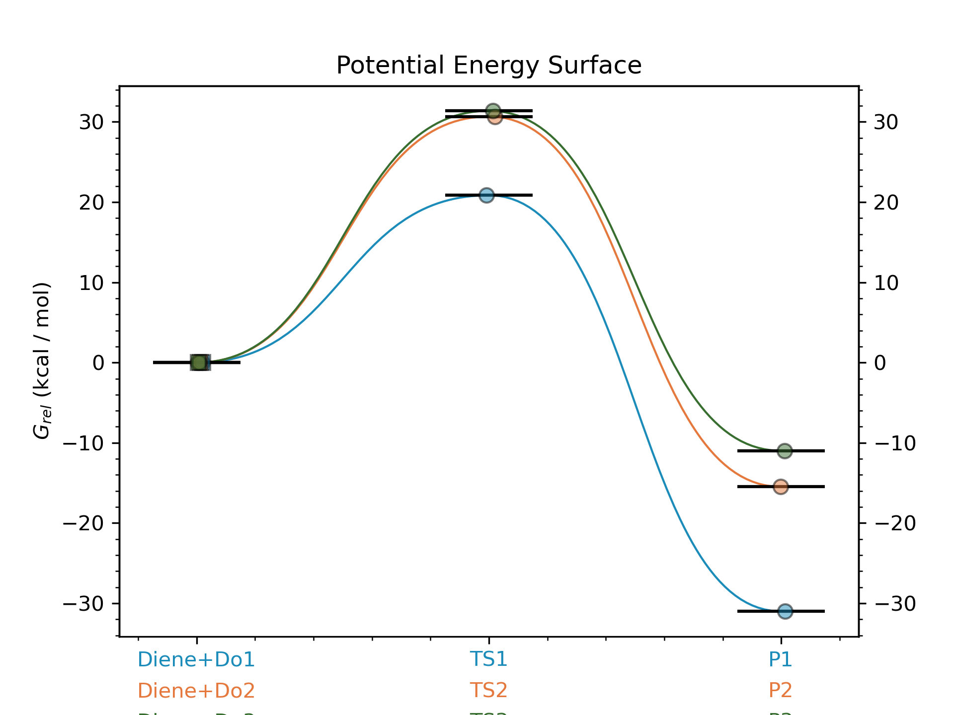
Specifially in this workflow we will calculate the free energy profile for the Diels-Alder reaction for three pairs of reactants shown below:
Reactants 1 |
Reactants 2 |
Reactants 3 |
C1=CC=CC1.C1=CC1 |
C1=CC=CC1.C1=CCC1 |
C1=CC=CC1.C1=CCCC1 |
|
|
|
Note
A jupyter notebook containing all the steps shown in this example can be found in the AQME repository in Github or in Figshare
Step 1: Importing AQME and other python modules
import os, glob, subprocess
import shutil
from pathlib import Path
from aqme.csearch import csearch
from aqme.qprep import qprep
from aqme.qcorr import qcorr
from rdkit import Chem
import pandas as pd
Step 2: Determining distance and angle constraints for TSs
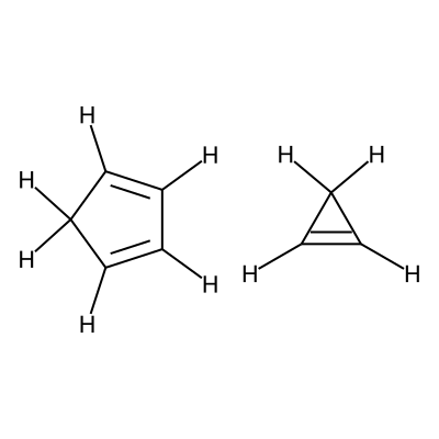
We visualize the first pair of reactants to be able to set up the constraints.
smi1 = 'C1=CC=CC1.C1=CC1'
mol1 = Chem.MolFromSmiles(smi1)
mol1 = Chem.AddHs(mol1)
for i,atom in enumerate(mol1.GetAtoms()):
    atom.SetAtomMapNum(i)
smi_new1 = Chem.MolToSmiles(mol1)
print('The new mapped smiles for checking numbers used in constraints is:', smi_new1)

mol1
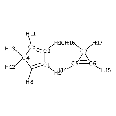
According to the image we will add the following constraints to the CSV, in the
constraints_dist column we will include [[3,5,2.35],[0,6,2.35]]
Note
For this step we are assuming that the code is being executed in a jupyter notebook. If it is being used through the python console, the following line allows to save the image with the mapping:
from rdkit.Chem import Draw
Draw.MolToFile(mol,'mapping_image.png')
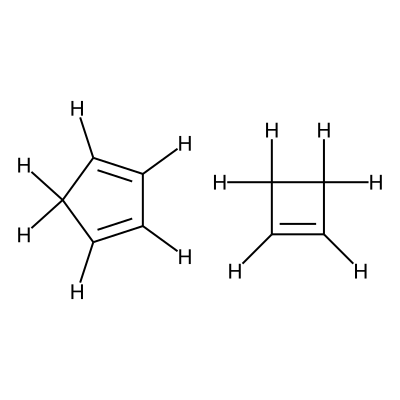
We visualize the second pair of reactants to be able to set up the constraints.
smi1 = 'C1=CC=CC1.C1=CCC1'
mol1 = Chem.MolFromSmiles(smi1)
mol1 = Chem.AddHs(mol1)
for i,atom in enumerate(mol1.GetAtoms()):
    atom.SetAtomMapNum(i)
smi_new1 = Chem.MolToSmiles(mol1)
print('The new mapped smiles for checking numbers used in constraints is:', smi_new1)

mol1
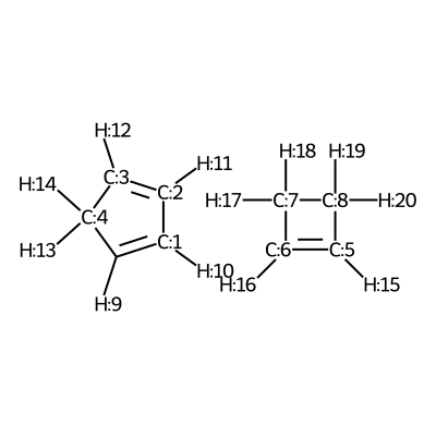
According to the image we will add the following constraints to the CSV, in the
constraints_dist column we will include [[3,6,2.35],[0,5,2.35]]
Warning
Although the atoms 5 and 6 are equivalent, we have observed that if we use
the same ordering as in the previous reaction for the constraints the TS
won't be found (i.e. with [[3,5,2.35],[0,6,2.35]]) whereas when we
use the constraints as shown in the example the TS is found.
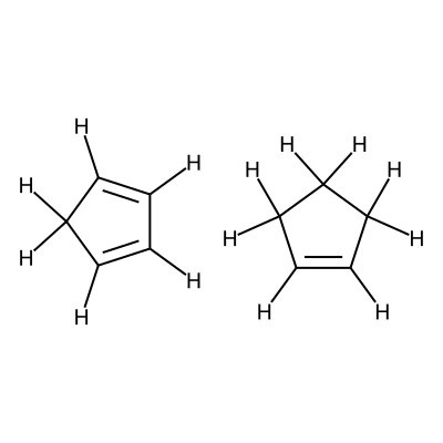
We visualize the third pair of reactants to be able to set up the constraints.
smi1 = 'C1=CC=CC1.C1=CCCC1'
mol1 = Chem.MolFromSmiles(smi1)
mol1 = Chem.AddHs(mol1)
for i,atom in enumerate(mol1.GetAtoms()):
    atom.SetAtomMapNum(i)
smi_new1 = Chem.MolToSmiles(mol1)
print('The new mapped smiles for checking numbers used in constraints is:', smi_new1)

mol1
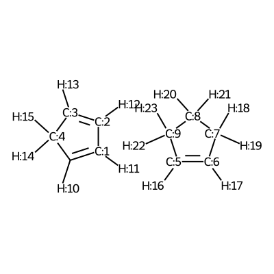
According to the image we will add the following constraints to the CSV, in the
constraints_dist column we will include [[3,5,2.35],[0,6,2.35]]
Step 3: CSEARCH conformational sampling
With the previous step we can now create a csv file containing all the molecules and noncovalent complexes to calculate, which will have the following contents:
SMILES,code_name,constraints_dist
C1=CC=CC1,Diene,
C1=CC1,Do1,
C1=CCC1,Do2,
C1=CCCC1,Do3,
C1([H:8])=[C:1]([H:9])[C:2]([H:10])=[C:3]([H:11])[C:4]1([H:12])[H:13].[C:5]1([H:14])=[C:6]([H:15])[C:7]1([H:16])[H:17],TS1,"[[3,5,2.35],[0,6,2.35]]"
C1([H:9])=[C:1]([H:10])[C:2]([H:11])=[C:3]([H:12])[C:4]1([H:13])[H:14].[C:5]1([H:15])=[C:6]([H:16])[C:7]([H:17])([H:18])[C:8]1([H:19])[H:20],TS2,"[[3,6,2.35],[0,5,2.35]]"
C1([H:10])=[C:1]([H:11])[C:2]([H:12])=[C:3]([H:13])[C:4]1([H:14])[H:15].[C:5]1([H:16])=[C:6]([H:17])[C:7]([H:18])([H:19])[C:8]([H:20])([H:21])[C:9]1([H:22])[H:23],TS3,"[[3,5,2.35],[0,6,2.35]]"
[C@H]1(C2C=CC3C2)[C@@H]3C1,P1,
[C@H]12[C@@H](C3C=CC2C3)CC1,P2,
[C@H]1(C2C=CC3C2)[C@@H]3CCC1,P3,
Now we can proceed to the conformer generation:
# read the CSV file with SMILES strings and constraints for TSs (from Step 2)
data = pd.read_csv('example2.csv')

csearch(input='example2.csv',
        program='crest',
        nprocs=12,
        cregen=True,
        cregen_keywords='--ethr 0.1 --rthr 0.2 --bthr 0.3 --ewin 1')
Step 4: Creating Gaussian input files for optimization and frequency with QPREP
program = 'gaussian'
mem='32GB'
nprocs=16

sdf_TS_files = glob.glob('CSEARCH/TS*crest.sdf')

# COM files for the TSs
qm_input_TS = 'B3LYP/def2tzvp opt=(ts,calcfc,noeigen,maxstep=5) freq=noraman'
qprep(files=sdf_TS_files,
      program=program,
      qm_input=qm_input_TS,
      mem=mem,
      nprocs=nprocs)

sdf_INT_files = glob.glob('CSEARCH/D*.sdf') + glob.glob('CSEARCH/P*.sdf')

# COM files for intermediates, reagents and products
qm_input_INT = 'B3LYP/def2tzvp opt freq=noraman'

qprep(files=sdf_INT_files,
      program=program,
      qm_input=qm_input_INT,
      mem=mem,
      nprocs=nprocs)
Step 5: Running Gaussian inputs for optimization and frequency calcs externally
Now that we have generated our gaussian input files (in the QCALC location of Step 3) we need to run the gaussian calculations. If you do not know how to run the Gaussian calculations in your HPC please refer to your HPC manager.
As an example, for a single calculation in Gaussian 16 through the terminal we would run the following command on a Linux-based system:
g16 myfile.com
Step 6: QCORR analysis
qcorr(files='QCALC/*.log',
      freq_conv='opt=(calcfc,maxstep=5)',
      mem=mem,
      nprocs=nprocs)
Step 7: Resubmission of unsuccessful calculations (if any) with suggestions from AQME
Now we need to run the generated COM files (in fixed_QM_inputs) with Gaussian like we did in Step 6
After the calculations finish we check again the files using QCORR
new_log_files = "QCALC/failed/run_1/fixed_QM_inputs/*.log"

qcorr(files=new_log_files,
      isom_type='com',
      isom_inputs='QCALC/failed/run_1/fixed_QM_inputs',
      nprocs=16,
      mem='32GB')
Step 8: Creating DLPNO input files for ORCA single-point energy calculations
program = 'orca'
mem='16GB'
nprocs=8

qm_files = os.getcwd()+'/QCALC/success/*.log' # LOG files from Steps 6 and 8
destination =  os.getcwd()+'/SP' # folder where the ORCA output files are generated

# keyword lines for ORCA inputs
qm_input = r'''
DLPNO-CCSD(T) def2-tzvpp def2-tzvpp/C
%scf maxiter 500
end
% mdci
Density None
end
% elprop
Dipole False
end'''.lstrip()

qprep(destination=destination,
      files=qm_files,
      program=program,
      qm_input=qm_input,
      mem=mem,
      nprocs=nprocs,
      suffix='DLPNO')
Step 9: Running ORCA inputs for single point energy calcs externally
Now we need to run the generated inp files (in sp_path) with ORCA (similarly to how we did in Step 4)
Step 10: Calculating PES with goodvibes
for this step we will need to have a yaml file to use as input for goodvibes. The contents of the yaml file are:
--- # PES
# Double S addition
   Reaction1: [Diene+Do1, TS1, P1]
   Reaction2: [Diene+Do2, TS2, P2]
   Reaction3: [Diene+Do3, TS3, P3]


--- # SPECIES
    Diene     : Diene*
   Do1     : Do1*
   TS1     : TS1*
   P1    : P1*
   Do2     : Do2*
   TS2     : TS2*
   P2    : P2*
   Do3    : Do3*
   TS3     : TS3*
   P3   : P3*


--- # FORMAT
   dec : 1
   units: kcal/mol
   dpi : 300
   color : #1b8bb9,#e5783d,#386e30
With this file we can now generate the profile.
# folder where the OUT files from Step 10 are generated
orca_files = os.getcwd()+'/SP/*.out'

# copy all the Gaussian LOG files and the ORCA OUT files into a new folder
# called GoodVibes_analysis (necessary to apply SPC corrections)

opt_files = glob.glob(qm_files)
spc_files = glob.glob(orca_files)
all_files = opt_files + spc_files

w_dir_main  = Path(os.getcwd())
GV_folder = w_dir_main.joinpath('GoodVibes_analysis')
GV_folder.mkdir(exist_ok=True, parents=True)

for file in all_files:
    shutil.copy(file, GV_folder)

# run GoodVibes
os.chdir(GV_folder)
command = 'python -m goodvibes --xyz --pes ../pes.yaml --graph ../pes.yaml -c 1 --spc DLPNO *.log'
subprocess.run(command.split())
os.chdir(w_dir_main)